Chapter 3. Handling IP Address Depletion
This chapter covers the following key topics:
- • Overview of IPv4 Addressing
An overview of the IPv4 class A/B/C addressing and basic subnetting concepts.- • Variable Length Subnet Mask (VLSM)
A description of variable length subnet masks and how they can be used in efficient assignment of the IP address space.- • IP Address Space Depletion
Through creative address allocation, supernetting, private addressing, and next generation protocols, the problem of IP address space depletion is being managed.- • Classless Interdomain Routing (CIDR)
CIDR, one of the major key elements of the Border Gateway Protocol 4 (BGP4), is used to control the growth of the global IP routing tables. Coverage includes a detailed description of different provider/customer addressing schemes in single and multihomed environments and tips about route aggregation.- • Private Addressing and Network Address Translation (NAT)
Network address translation software is used to map between private and global IP addresses.- • IP Version 6 (IPv6)
An overview of the IP next generation (IPng) addressing scheme and how it maps to the hierarchical model offered by CIDR and IPv4. - • Variable Length Subnet Mask (VLSM)
The overall model of address assignment continues to evolve. One of the major problems facing the Internet community is the depletion of IP addresses; this mandates the implementation of new IP addressing strategies. This chapter summarizes these strategies, their relative merits, and the issues surrounding address assignment on the Internet.
Addressing strategies are of direct and fundamental relevance to routing architecture. One of the basic functions of routing architecture and routers is to accommodate addresses for all the traffic that they direct. With the explosive growth of the Internet, the sheer number of addresses and the evolution of new addressing strategies have presented new challenges for routing architecture. Throughout this chapter, we will note particular routing rules and issues as they pertain to IP addressing.
This chapter begins with an overview of the basic IP addressing and subnetting models.
Overview of IPv4 Addressing
The IP addressing scheme that is widely used today is relevant to the IP version 4 (IPv4) implementation. This section discusses the following:
- • Basic Addressing [1]
- • Basic Subnetting [2]
- • Variable Length Subnet Mask (VLSM) [3]
- • Basic Subnetting [2]
Basic Addressing
The IP address, a 32-bit address, is represented by a dotted decimal notation of the form X.Y.Z.T (for example, 10.0.0.1). The 32-bit address field consists of two parts: a network number and a host number whose boundaries are defined based on the class of the IP address. The different IP classes are: A, B, and C1. This addressing scheme is sometimes referred to as the classfull model. The different classes lend themselves to different network configurations, depending on the desired ratio of networks to hosts. The full implications of the different classes will become more apparent as this chapter proceeds. For now, the chapter focuses on basic definitions of each class.
1Classes D and E for multicast and reserved addresses are beyond the scope of this book.
Class A Addressing
A class A network is represented by a 0 in the first bit. The first 8 bits (0-7) represent the network number, and the remaining bits (8-31) represent a host number on that network. The outcome of this representation, indicated in Figure 3-1, is 128 (27) class A network numbers having 16777216 (224) hosts per network (ignoring the boundaries such as all 0s and all 1s hosts that have special meaning). An example of a class A network is 10.0.0.1, representing network 10.0.0.0 and host 1.
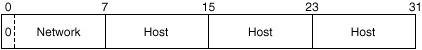
Figure 3-1 General class
A address format.
Class B Addressing
A class B network is represented by a 1 and a 0 in the first two bits. The first 16 bits (0-15) represent the network number, and the last 16 bits (16-31) represent the host number on that network. The outcome of this representation, indicated in Figure 3-2, is 16384 (214) network numbers with 655366 (216) hosts per network (also ignoring boundaries). An example of a class B network is 172.16.0.1 where 172.16.0.0 is the class B network, and 1 is the host.
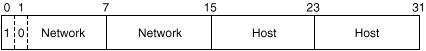
Figure 3-2 General class
B address format.
Class C Addressing
A class C network is represented by a 1 and a 1 and a 0 in the first three bits. The first 24 bits (0-23) represent the network number, and the last 8 bits (24-31) represent the host number on that network. The outcome of this representation, indicated in Figure 3-3, is 2097152 (221) network numbers with 256 (28) hosts per network (ignoring boundaries). An example of a class C network is 192.11.1.1, where 192.11.1.0 is the class C network and 1 is the host.
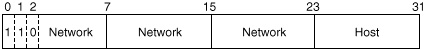
Figure 3-3 General class
C address format.
Basic Subnetting
Basic subnetting and variable length subnets are still quite misunderstood. This section first gives a brief introduction on how subnetting works and then tackles Variable Length Subnet Masks (VSLM), trying to make it as clear as possible.
A subnet or subnetwork is a subset of class A, B, or C networks. To elaborate more, take a closer look at IP addresses. IP addresses are formed of a network portion and a host portion. A network mask is used to separate the network information from the host information.
In figure 3-4, the network mask 255.0.0.0 is applied to network 10.0.0.0. The mask in a binary notation is a series of contiguous ones followed by a series of contiguous zeros. The ones portion represents the network number, whereas the zeros portion represents the host number. This would split the IP address 10.0.0.1 into a network portion of 10 and a host portion of 0.0.1. As such, classes A, B, and C each have what is called a natural mask, which is the mask created by the very definition of the network and host portions of each class.
- • Class A natural mask 255.0.0.0
- • Class B natural mask 255.255.0.0
- • Class C natural mask 255.255.255.0
- • Class B natural mask 255.255.0.0
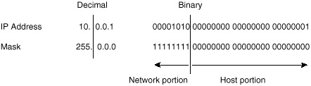
Figure 3-4 Basic
masking.
By separating the network and host portions of an IP address, masks facilitate the creation of subnets. Without the introduction of subnets, network numbers would be of very limited use. Each physical segment, such as an Ethernet, Token Ring, or FDDI segment, is normally associated with one or more network numbers. If this is the case, then a class A network of the form 10.0.0.0 would accommodate one physical segment with about 16 million hosts on it, as indicated in figure 3-5.
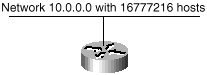
Figure 3-5 Illustration
of an unsubnetted class A address space.
With the use of masks, networks can be divided into subnetworks by extending the network portion of the address into the host portion. The subnetting technique increases the number of subnetworks and reduces the number of hosts.
In figure 3-6, a mask of 255.255.0.0 is applied to network 10.0.0.0. This will divide the IP address 10.0.0.1 into a network portion of 10, a subnet portion of 0, and a host portion of 0.1. The 255.255.0.0 mask has borrowed a portion of the host space and has applied it to the network space. As a result, the network space of the class 10 has increased from a single network 10.0.0.0 to 256 subnetworks ranging from 10.0.0.0 to 10.255.0.0. This would decrease the number of hosts per each subnet from 16777216 to 65536 (ignoring boundaries).

Figure 3-6 Basic
subnetting.
Variable Length Subnet Mask
The term Variable Length Subnet Mask (VLSM) refers to the fact that one network can be configured with different masks. The idea behind Variable Length Subnet Masks [3] is to offer more flexibility in dividing a network into multiple subnets while still maintaining an adequate number of hosts in each subnet. Without VLSM, one subnet mask only can be applied to a network. This would restrict the number of hosts given the number of subnets required. If you pick the mask such that you have enough subnets, you might not be able to allocate enough hosts in each subnet. The same is true for the hosts; a mask that allows enough hosts might not provide enough subnet space.
Suppose, for example, that you were assigned a class C network 192.214.11.0 and you need to divide that network into three subnets, with 100 hosts in one subnet and 50 hosts for each of the remaining subnets. Ignoring the two end limits 0 and 255, you theoretically have available to you 256 addresses 192.214.11.0 to 192.214.11.255. The desired subdivision cannot be done without VLSM, as you shall see.
There are a handful of subnet masks of the form 255.255.255.X that can be used to divide the class C network 192.214.11.0 into more subnets.
IP Address Space Depletion
The growing demand for IP addresses has put a strain on the classfull model, especially class B address space, which was getting depleted at a fast pace. Most companies requesting IP addresses have estimated that a class B would meet their requirement because it is a fair balance between the number of networks and the number of hosts. A class A was overkill with more than 16 million hosts, and a class C had too few hosts per network. By 1991, it was becoming obvious that the class B consumption was not slowing down and actions needed to be taken to prevent its depletion. Some of these measures consisted of creative assignment of IP addresses and promoting the use of private IP addresses for organizations that do not have global connectivity needs. Other measures resulted in the initiation of working groups and directorates such as the Routing and Addressing (ROAD) working group and the IP next generation (IPng) directorate. In 1992, the ROAD working group proposed the use of Classless Interdomain Routing (CIDR) as a measure to move away from classfull IP addressing. At the same time, the IPng directorate was working on developing a new and improved IP addressing scheme, IP version 6 (IPv6), that would eventually solve the problems that IPv4 is encountering.
The measures to handle the IP depletion can be grouped in the following categories:
- • Creative IP address space allocation
- • Classless Interdomain Routing (CIDR) [4]
- • Private addressing and Network Address Translation (NAT) [6,7]
- • IP version 6 (IPv6) [8]
- • Classless Interdomain Routing (CIDR) [4]
Along with depletion concerns, growing IP address demand generated a need to convert the IP addressing allocation process from a central registry. Originally, the Internet Assigned Numbers Authority (IANA) and the Internet Registry (IR) had total control for address assignment. IP addresses were assigned to organizations sequentially without any consideration of geographical factors and to how or where an organization would plug in into the Internet. This method had the effect of punching holes in the IP address space; that is, segregating individual or small numbers of IP addresses and eliminating large, contiguous ranges of numbers.
A different approach needed to be taken whereby a large, contiguous range of addresses is given to different administrations (such as service providers), and those providers in turn allocate addresses from their own space. In general, this funnel-down method of address allocation predicts a more controlled and hierarchical method of IP address distribution.
IP Address Allocation
Class A network numbers are limited resources, and the allocation from this space is restricted. Although the upper range of class A 64 to 127 will be distributed, there is still no definite plan on how this is going to be done.
Class B addresses are also restricted. They will be allocated only if the need for such addresses is fully justified. Due to the scarcity of class B network numbers and the under utilization of the address space by most organizations, the recommendation is to use multiple class Cs instead.
The class C network number space is now being divided and allocated in a way that is compatible with address aggregation techniques. Address aggregation is the practice of summarizing a contiguous block of addresses in a single notation, or advertisement. (Aggregation is also relevant to the CIDR model, to be discussed in the next section.)
Class C addresses are being distributed to ISPs with the requirement that the original allocation for the provider should last at least two years. In turn, each provider will allocate a block of addresses from its own range to each of its customers. Customers will not be granted more addresses from their ISPs until 80 percent of the original address space granted to the customer has been used. The allocation of class C addresses is illustated in table 3-1.
|
| |
|---|---|
| Organization Requirement | Address Assignment |
|
| |
| Fewer than 256 addresses | 1 class C network |
| Fewer than 512 but more than 256 | 2 contiguous class C networks |
| Fewer than 1,024 but more than 512 | 4 contiguous class C networks |
| Fewer than 2,048 but more than 1,024 | 8 contiguous class C networks |
| Fewer than 4,096 but more than 2,048 | 16 contiguous class C networks |
| Fewer than 8,192 but more than 4,096 | 32 contiguous class C networks |
| Fewer than 16,384 but more than 8,192 | 64 contiguous class C networks |
|
| |
If a subscriber has a requirement for more than 4,096 IP addresses, a class B network number might be allocated.
Organizations are encouraged to use Variable Length Subnet Mask (VLSM) as much as possible to use the address space more efficiently.
As far as the geographic allocation of blocks of C addresses, there are four major areas: Europe, North America, the Pacific Rim, and South and Central America. The allocation is summarized in table 3-2. The multiregional area represents network numbers that have been assigned prior to the implementation of this plan. Ranges designated as "Others" are for geographical areas other than the areas named specifically.
|
| |
|---|---|
| Area of Allocation | Address Spaces |
|
| |
| Multiregional | 192.0.0.0 to 193.255.255.255 |
| Europe | 194.0.0.0 to 195.255.255.255 |
| Others | 196.0.0.0 to 197.255.255.255 |
| North America | 198.0.0.0 to 199.255.255.255 |
| Central/South America | 200.0.0.0 to 201.255.255.255 |
| Pacific Rim | 202.0.0.0 to 203.255.255.255 |
| Others | 204.0.0.0 to 205.255.255.255 |
| Others | 206.0.0.0 to 207.255.255.255 |
|
| |
Classless Interdomain Routing (CIDR)
In recent years, the IP routing tables held in the Internet routers have grown in a way that caused routers to start being saturated as far as processing power and memory allocation. Statistics and growth rate projections suggest that routing tables have doubled in size every 10 months between 1988 and 1991. Figure 3-9 illustrates this growth. Without any plan of action, the routing table would have grown to about 80,000 routes in 1995. Actual data in 1996, however, showed that the routing table size is around 42,000 routes. This reduction in growth is attributed to the IP address allocation scheme discussed in the previous section and to the adoption of CIDR.

Figure 3-9 Routing table
growth chart.
CIDR is a move away from the traditional IP classes A/B/C. In CIDR, an IP network is represented by a prefix, which is an IP address and some indication of the leftmost contiguous significant bits within this address. For example, 198.32.0.0, which used to be an illegal class C network, is now a valid prefix with a notation 198.32.0.0/16. The /16 is an indication that you are using 16 bits of mask counting from the far left. This is similar to 198.32.0.0 255.255.0.0.
A network is called a supernet when the prefix boundary contains fewer bits than the network's natural mask. A class C network 198.32.1.0, for example, has a natural mask of 255.255.255.0. The representation 198.32.0.0 255.255.0.0 also represented as 198.32.0.0/16 has a shorter mask than the natural mask (16 < 24); hence, it is a supernet.
These address schemes are illustrated in figure 3-10.

Figure 3-10 CIDR-based
addressing illustration.
This notation enables you to lump all the more specific routes of 198.32.0.0 (such as 198.32.1.0 and 198.32.2.0, and so on) into one advertisement called an aggregate.
It is easy to be confused by all this new terminology, especially because the terms aggregate, CIDR block, and supernet are often used interchangeably in casual discussion. Generally, the terms all indicate that a list of contiguous IP networks has been summarized into one announcement. More precisely, CIDR is the <prefix,length> notation; supernets have a prefix length shorter than the natural mask; and aggregates indicate any summary route.
All the networks that are a subset of an aggregate or a CIDR block are called "more specific" because they give more information about the location of a network. More specific prefixes have a longer prefix length than the aggregate:
- • 198.213.0.0/16—aggregate of length 16
- • 198.213.1.0/20—more specific prefix of length 20
Routing domains that are CIDR-capable are called classless, in contrast to the traditional classfull routing domains. CIDR has depicted a new, more hierarchical Internet architecture, where each domain takes its IP addresses from a higher hierarchical level. This gives tremendous savings in route propagation especially when summarization is done close to the so-called leaf networks. Leaf networks are endpoints on the global network; they do not, in turn, provide Internet connection to other networks. An ISP that supports numerous leaf networks subdivides its subnets into many smaller blocks of addresses to serve those customers. Aggregation permits the ISP to advertise the addresses in a single notation rather than many, thus resulting in more efficient routing strategies and propagation.
The efficiency of aggregation is illustrated in figure 3-11. In this example, ISP3 has been given the block 198.0.0.0 through 198.255.255.0. ISP3 has given two blocks of its addresses to ISP1 and ISP2. ISP1 has the range 198.32.0.0 through 198.32.255.0, and ISP2 has the range 198.33.0.0 through 198.33.255.0. In the same manner, ISP1 and ISP2 have allocated their own customers a block of addresses from their own ranges. The left side instance of figure 3-11 shows what happens if you do not use CIDR: ISP1 and ISP2 would have to advertise all the subnets coming from their customers, and ISP3 would have passed all these advertisements to the outside world. This would result in a major increment in the global IP routing tables.
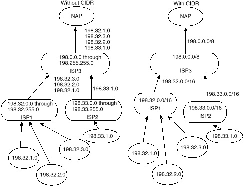
Figure 3-11 Comparison of
classful addressing and CIDR-based addressing.
The right side instance of figure 3-11 shows the same scenario when CIDR is applied. ISP1 and ISP2 are performing aggregation on their customer subnets, ISP1 is advertising the aggregate 198.32.0.0/16, and ISP2 is advertising the aggregate 198.33.0.0/16. In the same manner, ISP3 is performing aggregating on its customer subnets, ISP1 and ISP2, and is sending only one aggregate 198.0.0.0/8. This results in tremendous savings in the global IP routing tables.
As you can see, aggregation results in more significant efficiency gains when done close to the leaf node because the majority of the subnets to be aggregated are deployed at the customer premises. Aggregation at higher levels, such as ISP3, results in less reduction because it is dealing with fewer networks to start with.
Aggregation works optimally if every customer connects to his provider via one connection only (a scenario called single-homing), and also if the customer has taken its IP addresses from its provider's prefixes. Unfortunately, this is not always the case in the real world. Situations arise, for example, where customers already have IP addresses that do not belong to their provider's range. As another example, some customers (who could be providers themselves) have found the need to connect to multiple providers at the same time (a scenario known as multihoming). These situations result in further complications and less flexibility in aggregation.
These complications to aggregation are discussed in more detail. But first, it is important to understand a couple of routing rules, as described in the next two subsections.
The Longest Match Routing Rule
Routing to all destinations is always done on a longest match basis: a router that has to decide between two different length prefixes of the same network will always follow the longer mask. Suppose, for example, that a router has the following two entries in its routing table:
- -198.32.1.0/24 via path 1
- -198.32.0.0/16 via path 2
When trying to deliver traffic to host 198.32.1.1, the router tries to match the destination with the longest prefix and would deliver the traffic via path 1. This is illustrated in figure 3-12 where Domain C is receiving the two updates 198.32.1.0/24 and 198.32.0.0/16; traffic toward 198.32.1.1 is following path 1. In case path 1 goes down for some reason, traffic will take path 2. In cases where Domain C is receiving identical routing updates with masks of equal length coming from Domain A and Domain B, Domain C would pick one path or the other or both depending on the load balancing techniques offered by the specific routing implemetation defined for that domain.
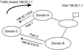
Figure 3-12 Following the
longest match.
The longest match rule implies that destinations connected to multiple domains must always be explicitly announced—that is, announced in their most specific, not aggregate, forms—by these domains. In figure 3-12, because Domain B does not explicitly advertise route 198.32.1.0/24, traffic from the customer to the host must always go via the longest prefix match, through Domain A. Such a routing configuration might put an unacceptable burden on Domain A.
Less Specific Routes of a Network's Own Aggregate
A specific rule of routing states that, for the sake of preventing routing loops, a network must not follow a less specific route for a destination that matches one of its own aggregated routes. A routing loop occurs when traffic circles back and forth between domains, never reaching its final destination. Default routes 0.0.0.0/0.0.0.0 are a special case of this rule. A network should not follow the default to destinations that are part of one of its aggregated advertisements. This is why routing protocols that handle aggregation of routes should always keep a Pit Bucket (Null0 route in Cisco's terminology) to the aggregate route itself. Traffic sent to the pit bucket will be dropped, which would stop the loop situation.
Troubleshooting:
Avoiding loops in default routing by use of pit buckets.
Figure 3-13 illustrates ISP1 aggregating its domain into a single route 198.32.0.0/13. Assume that the link between ISP1 and its customer Samnet (where network 198.32.1.0/24 exists) broke. Suppose also that ISP1 has a default route 0.0.0.0/0.0.0.0 that points to ISP2 for addresses not known within ISP1. Traffic toward 198.32.1.1 will follow the aggregate route to ISP1, will not find the destination, and will follow the default route back to ISP2. The traffic will bounce back and forth between ISP2 and ISP1. To prevent such a loop, a null0 entry to the aggregate route, installed in ISP1's border router will drop all packets destined to an unreachable destination less specific than the aggregate route.

Figure 3-13 Following
less specific routes of a network's own aggregate causes loops.
Aggregation, if not properly applied, could result in routing loops and black holes. A black hole occurs when traffic reaches and stops at a destination that is not its intended destination, but from which it cannot be forwarded. These and other routing challenges will become more apparent as you learn about multiple IP address allocation schemes and how they interact with aggregation.
Single-Homing Scenario: Addresses Taken from Outside the Provider's Address Space
In this scenario, the customer is connected to a single provider and has an IP address space totally different from the provider's. This could have happened because the customer changed providers and kept the addresses of the previous provider. Usually in this situation, customers are encouraged or forced to renumber. But if renumbering does not take place, the new provider cannot aggregate the customer addresses. Moreover, the old provider cannot aggregate as efficiently as it once did, because a hole has been punched in its address space. The overall effect of using addresses from outside the provider's address space is that more routes must be installed in the global routing tables.
Multihoming Scenario: Addresses Taken from One Provider
In this scenario, customers are connected to multiple providers. Customers are small enough that they need to take IP addresses from only one of their multiple providers. We will consider two ISPs, ISP1 and ISP2, and their customers: Jamesnet, Stubnet, and Lindanet. The IP address ranges for each domain, corresponding aggregate, and provider are listed in table 3-3.
|
| ||||
|---|---|---|---|---|
| Domain | Address Range | Aggregate | Provider | Address Taken From |
|
| ||||
| ISP1 | 198.24.0.0-198.31.0.0 | 198.24.0.0/13 | ||
| Jamesnet | 198.24.0.0-198.24.15.0 | 198.24.0.0/20 | ISP1, ISP2 | ISP1 |
| Stubnet | 198.24.16.0-198.24.23.0 | 198.24.16.0/21 | ISP1 | ISP1 |
| Lindanet | 198.24.56.0-198.24.63.0 | 198.24.56.0/21 | ISP1, ISP2 | ISP1 |
| ISP2 | 198.32.0.0-198.39.0.0 | 198.32.0.0/13 | ||
|
| ||||
Note that Jamesnet and Lindanet are multihomed to ISP1 and ISP2 with their address ranges taken from ISP1. Stubnet is single-homed to ISP1 with an address range taken from ISP1. This is illustrated in figure 3-14.
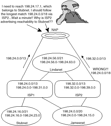
Figure 3-14 ISP2
advertising the wrong aggregate causes black holes.
Advertising aggregates is a tricky business. Customers and ISPs have to be careful about the IP address ranges that the aggregate covers. No one is allowed to aggregate someone else's routes (proxy aggregation) unless the aggregating party is a superset of the other party or both parties are in total agreement. In the following, you will see how ISP2 can cause a routing black hole by aggregating the ranges coming from Jamesnet and Lindanet.
Troubleshooting:
Black holes that result from inappropriate aggregation of others' routes.
If ISP2 were to send an aggregate that summarizes Jamesnet and Lindanet into one update (198.24.0.0/18), then a routing black hole will occur. Stubnet, for example, which is a customer of ISP1, has an IP address space that falls inside the aggregate 198.24.0.0/18. If ISP2 were to advertise that aggregate, then traffic to Stubnet will follow the longest match and end up in ISP2. This is why ISP2 will have to specifically list each of the IP address ranges that it has in common with ISP1 on top of its own address space 198.32.0.0/13.
Figure 3-15 shows the correctly advertised aggregates. ISP2 has to advertise the aggregates from Jamesnet and Lindanet explicitly. This way, traffic advertised to Stubnet would never go to ISP2.
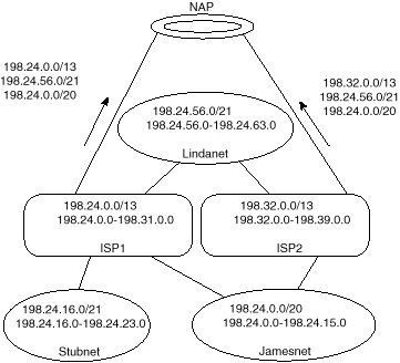
Figure 3-15 Correctly
advertised aggregates.
Note in figure 3-15 that ISP1 is also advertising the explicit aggregates of Jamesnet and Lindanet. If ISP1 were to advertise the less-specific aggregate 198.24.0.0/13 only, all traffic toward Jamesnet and Lindanet would always follow the longest match via ISP2.
Multihoming Scenario: Addresses Taken from Different Providers
One possibility for large domains is to take addresses from different providers based on the geographic location. Consider figure 3-16. Largenet has taken its IP addresses from two different providers, ISP1 and ISP2. With this design, each provider will be able to aggregate its own address space without having to list specific ranges from the other provider. ISP1 would advertise the aggregate 198.24.0.0/13, and ISP2 would advertise the aggregate 1928.32.0.0/13. Both aggregates are supersets of an IP address block in Largenet.

Figure 3-16 Multihomed
environment with addresses from different providers.
The major drawback with the design illustrated in figure 3-16 is that backup routes to multihomed organizations are not maintained. ISP2 is advertising only its block of addresses and not the block taken from ISP1. In case ISP1 has problems and the 198.24.0.0/13 is lost, traffic to Largenet destined for 198.24.0.0/20 will be affected because it is not advertised anywhere else. The same reasoning applies for Largenet's addresses taken from ISP2. If the link to ISP2 fails, accessibility of the 198.32.0.0/20 range will be impaired. To remedy this situation, ISP1 has to advertise 198.32.0.0/20 and ISP2 has to advertise 198.24.0.0/20.
Multihoming Scenario: Addresses Taken from None of the Providers
Figure 3-17 illustrates a situation in which addresses are taken from a range totally different from ISP1 or ISP2's address space. In this case, both ISP1 and ISP2 will advertise a specific aggregate (204.24.0.0/20) on top of their own ranges (198.24.0.0/13 and 198.32.0.0/13). The drawback of this method is that all routers in the Internet must have a specific route to the new range that is introduced. Too many of such instances would result in an increase in the overall routing tables.
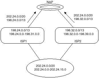
Figure 3-17 Addresses
obtained outside ISP address space.
Aggregation Recommendations
In conclusion, a domain that has been allocated a range of addresses has the sole authority for aggregation of its address space. When a domain performs aggregation, it should aggregate as much as possible without causing ambiguity such as is possible in the case of multihomed networks.
Different situations require different designs. No one specific solution can handle all cases. It is recommended that single-homed customers obtain a single contiguous prefix from the direct provider. If they change providers, a plan should be put in place to transition the addressing to the new provider's address space. For multihomed customers, address assignments should be done in a way to maximize aggregation as much as possible. In the case where aggregation impacts redundancy, redundancy should prevail even if extra networks have to be listed.
The introduction of CIDR has helped damper the explosion of global routing tables tremendously over the last few years. The Border Gateway Protocol 4 (BGP4) is the routing protocol of choice on the Internet in part because it so efficiently handles route aggregation and propagation between different autonomous systems. As this book progresses, you will see more and more examples of the importance of CIDR in controlling traffic behavior and stability.
To find ways to slow down the pace at which the IP addresses were being allocated, it was important to identify different connectivity requirements and try to assign IP addresses accordingly.
Most organizations' connectivity needs fall in the following categories:
- • Global connectivity
- • Private connectivity (total or partial)
Global Connectivity
Global connectivity means that hosts inside an organization have access to both internal hosts and Internet hosts. In this case, hosts have to be configured with globally unique IP addresses that are recognized inside and outside the organization. Organizations requiring global connectivity must request IP addresses from their service providers.
Private Connectivity
Private connectivity means that hosts inside an organization have access to internal hosts only, not Internet hosts. Examples of hosts that require only private connectivity include bank ATM machines, cash registers in a retail company, or any host that does not really need to reach or be reached by hosts outside the company. Private hosts need to have IP addresses that are unique inside the organization, but do not have to be unique outside the organization. For this type of connectivity, the IANA has reserved the following three blocks of the IP address space for what is referred to as "private Internets:"
- • 10.0.0.0 through 10.255.255.255 (a single
class A network number)
- • 172.16.0.0 through 172.31.255.255 (16 contiguous class B network numbers)
- • 192.168.0.0 through 192.168.255.255 (256 contiguous class C network numbers)
- • 172.16.0.0 through 172.31.255.255 (16 contiguous class B network numbers)
An enterprise that picks its addresses from the preceding range does not need to get permission from the IANA or an Internet Registry. Hosts that get a private IP address can connect with any other host inside the organization, but cannot connect to hosts outside the organization without going through a proxy gateway. The reason is that IP packets leaving the company will have a source IP address that is ambiguous outside the company and cannot be replied to by outside hosts. Because multiple companies building private networks can use the same IP addresses, fewer unique global IP addresses need to be assigned.
Hosts having private addresses can co-exist with hosts having global addresses. Figure 3-18 illustrates such an environment. Companies might choose to have most of their hosts private and still keep particular segments with hosts having global addresses. The latter hosts can reach the Internet as usual. Companies that use private addresses and still have connectivity to the Internet have the responsibility of applying routing filters to prevent the private networks from being leaked to the Internet.
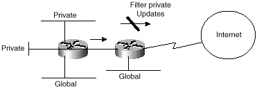
Figure 3-18 General
private Connectivity environment.
The drawback of this approach is that if an organization later on decides to open up its hosts to the Internet, the private IP addresses will have to be renumbered.With the introduction of new protocols such as the Dynamic Host Configuration Protocol (DHCP) [5], this task might become easy. DHCP provides a mechanism for transmitting configuration parameters (including IP addresses) to hosts using the TCP/IP protocol suite. Provided that the hosts are DHCP-compatible, hosts can get their new addresses dynamically from a central server.
Hosts that have private addresses can still reach the outside by going through a gateway or some kind of host that has a global address.
Host A in Figure 3-19 has a private IP address. If A wants to telnet to a destination outside the company, it can do so by first logging into host B and then telnetting from host B to the outside. Packets leaving the company now would have B's source IP address, which is global and can be replied to.
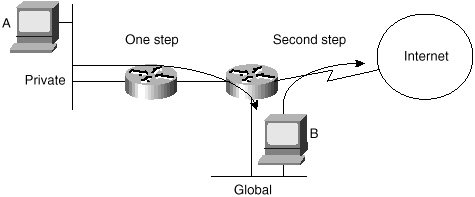
Figure 3-19 Privately
addressed hosts accessing Internet resources.
Network Address Translator
Companies migrating from a private address to a global address space can do so with the help of Network Address Translators (NAT). Cisco Systems offers this solution as part of its Cisco Internetwork Operating System (IOS)™ software running on its routers.
NAT technology enables private networks to connect to the Internet without resorting to renumbering IP addresses. A NAT router is placed at the border of a domain, and it translates the private addresses into global addresses before sending packets to the Internet.
As illustrated in figure 3-20, hosts A and B have private IP addresses 10.1.1.1 and 10.1.1.2. If A and B want to reach destinations outside the company, the NAT will convert the source IP addresses of the packets according to the predefined mapping in the NAT table. Packets from host A will reach the outside with a source IP address of 128.213.x.y, and packets from host B will reach the outside as coming from source IP address 128.213.z.w. Hosts in the global domains will not know the difference and will reply to hosts A and B as they would to any other host. On the way back, the destination address of the packets will be mapped back to the private IP address.
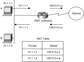
Figure 3-20 Network
Address Translator example.
Discussions about NAT devices are beyond the scope of this book because they have to handle many "corner cases" and more involved situations. Such cases include enterprises that have used addresses that are not part of the IANA private addresses. In this case, addresses used could be already assigned by the IANA to some other company. Other situations involve enterprises that get assigned fewer global addresses than their number of hosts. In this case, the NAT has to dynamically map private IP addresses to a smaller pool of global addresses.
IP Version 6 (IPv6)
IP version 6 (IPv6), also known as IP next generation (IPng), is a move to improve the existing IPv4 implementation.
The IPng proposal was released in July 1992 at the Boston Internet Engineering Task Force (IETF) meeting, and a number of working groups were formed in response. IPv6 tackles issues such as the IP address depletion problem, quality of service capabilities, address autoconfiguration, authentication, and security capabilities.
IPv6 is still in its experimentation stage. It is not easy for companies and administrators deeply invested in the IPv4 architecture to migrate to a totally new architecture. As long as the IPv4 implementation keeps providing hooks and techniques (as cumbersome as they might be) to tackle all the major issues that IPv6 will solve, adopting IPv6 might not seem very compelling to many companies. How soon or how late people will migrate to IPv6 is yet to be seen.
As far as this book is concerned, we will only touch on part of the IPv6 addressing scheme and how it compares to what you already have seen in IPv4.
The IPv6 addresses are 128 bits long (compared to 32 bits in IPv4). This should provide ample address space to handle scalability issues in the Internet (128 bits of addressing will translate into 2128—which is a lot of addresses).
The types of IPv6 addresses are indicated by the leftmost bits of the address in a variable length field called the Format Prefix (FP). This is illustrated in figure 3-21.
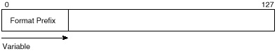
Figure 3-21 IPv6 prefix
and address format.
Table 3-4 outlines the initial allocation of these prefixes. IPv6 has defined multiple types of addresses; we are interested in the provider-based unicast addresses and the local use addresses for comparison with IPv4 techniques.
|
| |
|---|---|
| Description | Format Prefix |
|
| |
| Reserved | 0000 0000 |
| Unassigned | 0000 0001 |
| Reserved for NSAP Allocation | 0000 001 |
| Reserved for IPX Allocation | 0000 010 |
| Unassigned | 0000 011 |
| Unassigned | 0000 1 |
| Unassigned | 0001 |
| Unassigned | 001 |
| Provider-Based Unicast Address | 010 |
| Unassigned | 011 |
| Reserved for Geographic Unicast Addresses | 100 |
| Unassigned | 101 |
| Unassigned | 110 |
| Unassigned | 1110 |
| Unassigned | 1111 0 |
| Unassigned | 1111 10 |
| Unassigned | 1111 110 |
| Unassigned | 1111 1110 0 |
| Link Local Use Addresses | 1111 1110 10 |
| Site Local Use Addresses | 1111 1110 11 |
| Multicast Addresses | 1111 1111 |
|
| |
Provider-Based Unicast Addresses
Provider-based unicast addresses are similar to the IPv4 global addresses. The format of these addresses is illustrated in figure 3-22. Descriptions of the address fields are as follows:
- • Format Prefix—First three bits are
010, indicating a provider-based unicast address.
- • REGISTRY ID—Identifies the Internet address registry that assigns the PROVIDER ID.
- • PROVIDER ID—Identifies the service provider responsible for this address.
- • SUBSCRIBER ID—Identifies which subscriber is connected to the service provider.
- • SUBNET ID—Identifies the physical link to which the address belongs.
- • INTERFACE ID—Identifies a single interface among interfaces that belong to the SUBNET ID. For example, this could be the traditional 48-bit IEEE-802 Media Access Control (MAC) address.
- • REGISTRY ID—Identifies the Internet address registry that assigns the PROVIDER ID.

Figure 3-22 IPv6 address
assignment hierarchy.
The IPv6 global address incorporates the CIDR functions of the IPv4 scheme. Addresses are defined in such a way as to allow hierarchy, where each entity takes its portion of the address from an entity above it, as illustrated in figure 3-23.
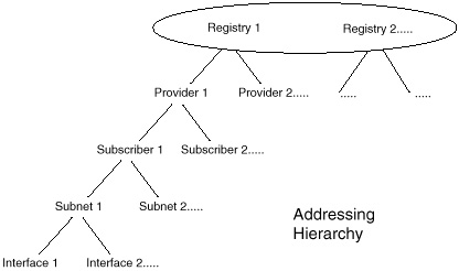
Figure 3-23 IPv6 address
assignment hierarchy.
Local-Use Addresses
Local-use addresses are similar to the IPv4 private addresses defined in RFC 1918. Local-use addresses are divided into two types: Link-Local Use (prefix 1111111010), which are private to a particular physical segment, and Site-Local Use (prefix 1111111011), which are private to a particular site. Figure 3-24 illustrates the format of these local use addresses.

Figure 3-24 Local-use
address formats.
The local-use addresses have local meaning. The link addresses have local meaning to a particular segment, and the site addresses have local meaning to a particular site.
Companies that are not connected to the Internet can easily assign their own addresses without a need for requesting prefixes from the global address space. If the company later decides to interconnect globally over the Internet, a REGISTRY ID, PROVIDER ID, and SUBSCRIBER ID will be assigned to be used with the already assigned local addresses. This is a major improvement over having to replace all private addresses with global addresses or using Network Address Translation tables to get things working in the IPv4 addressing scheme.
Looking Ahead
IP addresses and addressing schemes are basic elements of interdomain routing. Addressing by itself defines where certain information can be found, but does not give any indication on how the information is to be accessed. A mechanism is needed to exhange information about destinations and to calculate the optimal way to reach a certain destination. This mechanism, of course, is routing.
This chapter concludes all the foundation material required before proceeding to study routing architecture itself. In the next chapter, the basics of interdomain routing are covered, building on concepts of addressing, global networks, and domains as discussed in this and previous chapters. Routing protocols in general, and BGP in particular, are discussed, with implementation details on BGP to follow in Chapter 5 and beyond.
References
[1] RFC 791 Internet Protocol (IP)
[2] RFC 917 Internet Subnets
[3] RFC 1878 Variable Length Subnet Table for IPv4
[4] RFC 1519 Classless Interdomain Routing (CIDR)
[5] RFC 1541 Dynamic Host Configuration Protocol
[6] RFC 1918 Address Allocation for Private Internets
[7] RFC 1631 The IP Network Address Translator (NAT)
[8] RFC 1884 IP Version 6 Addressing Architecture